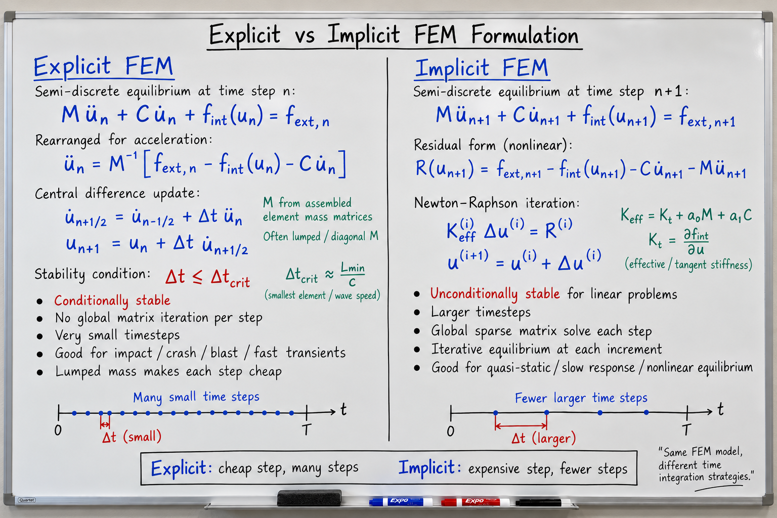
Implicit and explicit finite element solvers can often model the same physical system, but they reach the solution in different ways. The most appropriate choice depends on the event timescale, the nature of the non-linearity and the information required from the analysis.
The basic distinction
Implicit analysis is commonly used for static and quasi-static structural problems. The solver establishes equilibrium at successive load increments, with non-linear problems typically requiring iterations as contact conditions, stiffness and material behaviour evolve.
Explicit analysis is particularly well suited to short-duration dynamic events such as impact, crash and blast, especially where severe deformation, changing contact or material failure occurs. Rather than performing global equilibrium iterations, the solver calculates acceleration from the current forces and mass, then advances the motion through small time increments.
Implicit for statics, explicit for dynamics — is it that simple?
Neither method is restricted to those applications. Implicit solvers can perform transient dynamic analyses, while explicit solvers can assess quasi-static behaviour when inertial and strain-rate effects are appropriately controlled.
The distinction is therefore one of numerical strategy, not simply whether the loading is static or dynamic. One approach may be substantially more efficient or robust for a particular problem.
Where implicit analysis is usually strongest
Implicit analysis is generally well suited to static and quasi-static assessments, where inertial effects are negligible and the objective is to establish structural equilibrium.
Typical applications include static strength and stiffness assessments of civil structures, infrastructure products and pressure-loaded equipment. These assessments can include substantial material, geometric and contact non-linearity.
When convergence is well behaved, implicit solvers can use relatively large load increments, providing an efficient route to predicting stresses, deflections and load-carrying capacity. For rate-independent static problems, those increments describe the progression of loading rather than the passage of physical time.
The challenge: convergence
Abrupt changes in contact, material softening, buckling and large deformation can make equilibrium iterations difficult. Smaller load increments or a different solution strategy may be needed to follow the response.
Convergence difficulties do not automatically mean that the underlying physics cannot be represented. However, they may reflect either a numerical difficulty or a genuine structural instability, so the cause needs to be investigated rather than treated solely as a solver problem.
Where explicit analysis is usually strongest
Explicit methods are particularly effective for short-duration, highly non-linear events involving rapidly changing contact, large deformation and failure. Crash, impact, blast, drop and penetration assessments are common applications, alongside complex events such as vehicle rollover.
Avoiding global equilibrium iterations can be advantageous when contact repeatedly opens and closes or structural geometry changes significantly. The trade-off is the stability limit: each increment is relatively inexpensive, but completing the simulation may require a very large number of small time steps.
The stable time step matters
For many explicit structural analyses, an element's stable time step can be estimated from the time required for a stress wave to cross it:
Element time step ≈ Characteristic length ÷ Material wave speed
The wave speed depends on the material's effective stiffness and density. The characteristic length depends on the element geometry and formulation.
For a homogeneous material with comparable element formulations and material states, wave speeds are generally similar throughout the mesh. The element with the smallest characteristic length will therefore typically impose the most restrictive element time step.
In a multi-material model, the governing factor is the combination of characteristic length and wave speed. A larger element can impose a smaller time step if its material wave speed is sufficiently high.
This is an approximate explanation rather than a universal calculation rule. Solver safety factors, contact formulations and other model features can also affect the permitted time step. The limit may also change as elements deform and material behaviour evolves.
Even a single unnecessarily small element can significantly increase computational cost. Initially well-shaped elements can also become heavily distorted during loading, reducing their characteristic lengths and slowing the analysis. Efficient explicit modelling therefore requires both an appropriate initial mesh resolution/ quality and attention to how that mesh behaves throughout the event.
Can explicit analysis be used for quasi-static problems?
Yes. Explicit solvers can be effective for challenging quasi-static problems, particularly where complex contact, material failure or instability makes implicit convergence difficult.
To reduce computational cost, loading may be applied faster than the physical process. However, the accelerated loading must not introduce significant inertial effects or alter rate-dependent behaviour relevant to the assessment.
Rapid load application and changing contact can also introduce oscillations into the results. These should be investigated rather than assumed to be harmless noise.
Energy histories, reaction forces, deformation modes and sensitivity to loading duration should be examined together. The aim is to establish that the predicted response represents the intended quasi-static behaviour, rather than an unintended dynamic event.
Can implicit analysis be used for dynamic problems?
Yes. Implicit transient dynamic analysis accounts for inertia and, where applicable, damping alongside the internal structural forces. For non-linear problems, the solver typically iterates within each time increment to satisfy dynamic equilibrium between these contributions and the applied loading.
Implicit dynamics is not necessarily restricted to low-frequency response, but its ability to resolve higher frequencies depends on the time increment, spatial discretisation and integration scheme.
Large time increments can inadequately resolve higher-frequency behaviour, while numerical damping may suppress it. A solution can therefore remain numerically stable without accurately capturing all the response of interest.
Time increments and integration settings must be selected to resolve the relevant loading and structural response, not simply to obtain a stable solution.
A useful decision framework
Is the response dominated by equilibrium?
Static and slowly varying structural problems generally favour implicit analysis when inertial effects are negligible.
Is the event short and strongly dynamic?
Impact, crash and blast often favour explicit integration, particularly when combined with complex contact and large deformation.
Are severe contact changes or failure expected?
Explicit analysis may offer greater robustness where changing contact, collapse or failure makes implicit equilibrium iterations difficult.
Does the time-dependent response need to be resolved?
When acceleration, vibration or wave propagation matters, the analysis must resolve the relevant timescales and frequencies. Both methods can do this; the choice depends on the event duration, non-linearity and computational cost.
The practical answer
Static or quasi-static loading → Implicit is usually preferable.
Short-duration, highly dynamic loading → Explicit is often preferable.
Severe contact, deformation or failure → Explicit may offer a more robust solution, including for some quasi-static problems.
Both approaches can represent non-linear and dynamic behaviour. The most suitable choice balances the physics, the required results and computational efficiency.